20.080.RiOS.CS · rideOS research project · NUS High School
| Student | Kristofer Tsai |
|---|---|
| School | NUS High School |
| External Mentor | Allison Liemhetcharat, rideOS |
| NUS High Teacher Mentor | Chiam Sher-Yi |
| Project Purpose | Investigate how machine learning methods can better predict NBA game outcomes. |
| Methods | API data extraction, data reformatting, feature engineering, and WEKA classifier analysis. |
Abstract
There are 30 teams in the National Basketball Association (NBA). To predict the outcome of an NBA game, previous research has used methods including adversarial synergy graph models, entropy-based principles, and neural-network regression. This project uses Waikato Environment for Knowledge Analysis (WEKA), an open-source machine learning platform, to study NBA team statistics with a range of machine learning methods. Compared with approaches that study game scores alone, isolating specific team statistics allows for a more detailed analysis of individual NBA games. Classification via Regression and J48 produced the strongest F-measure scores when using recent Game Result as a single attribute. Across the displayed tests, adding multiple features did not improve performance consistently across classifiers.
Introduction
The National Basketball Association (NBA) has 30 teams: 29 in the United States and 1 in Canada. It is one of the four major professional sports leagues in North America and the premier men's professional basketball league in the world. In each game, a lineup of five players from the home team competes against five players from the away team. To win, a team must outscore its opponent by creating higher-quality shots, defending effectively, and managing possessions.
Basketball outcomes are influenced by many factors, including player ability, team coordination, coaching strategy, physical condition, and equipment quality. This creates a high level of uncertainty. Unexpected moments are common in the NBA, such as JR Smith running out the clock in Game 1 of the 2018 NBA Finals or Tracy McGrady scoring 13 points in 35 seconds against the San Antonio Spurs in 2004.
Nevertheless, previous game performance can reveal relationships that help predict future outcomes. In the 2018 NBA Finals between the Golden State Warriors and Cleveland Cavaliers [1], the Warriors performed better across many statistics, including effective field goal percentage, and had a lower turnover rate through the first three games. Up 3-0, the statistics strongly suggested a Warriors sweep, and betting markets reflected that confidence. The Warriors went on to defeat the Cavaliers 108-85 in Game 4 and win the championship.
This paper identifies relationships between specific NBA game statistics and future game outcomes. The process involved extracting data from a reliable NBA source, reformatting it into comma-separated values (CSV) for WEKA [2], and repeatedly testing feature combinations across classifiers. Results were measured using F-measure [3], which is described later. Most F-measure results fell between the mid-0.5 and low-0.6 range.
Methodology
To predict NBA game outcomes with machine learning, this project studied the relationships between detailed basketball statistics and game results. The methodology has three main steps:
- Extracting the data
- Reformatting the data
- Analysing the data in WEKA
The data was extracted through a third-party API that provided access to an NBA data library. The extracted data was returned in JavaScript Object Notation (JSON), but WEKA requires comma-separated values (CSV). As a result, the data had to be reformatted before analysis. Different combinations of parameters and attributes were then tested to study the relationship between statistics and game outcomes.
Data extraction was completed using API-NBA [4], a freemium API developed by API-SPORTS and verified by the RapidAPI community. Using Python, 1,231 requests were sent to extract game data from the 2018–2019 NBA season. Of those requests, 1,219 were successful. Game IDs 4640–4650 and 5065 returned blank results, but the missing games should not significantly affect the experiment because the sample size remains large.
The JSON data was flattened and saved as a CSV file using Python. Converting JSON into CSV removes some hierarchical structure, but it makes the data more compact and easier for WEKA to process. Appendix A shows examples of both formats.
The final CSV file contained 54 attributes, listed in Appendix B. To compare home and away team statistics, Excel was used to calculate difference attributes by subtracting the away-team value from the home-team value. For example, PointsInPaintDiff = HomePointsInPaint - AwayPointsInPaint. This produced 26 new difference attributes.
Each of the 26 new attributes was first tested individually using a J48 tree to predict the game outcome. J48 is WEKA’s open-source Java implementation of the C4.5 decision-tree algorithm developed by Ross Quinlan. It was selected as the starting classifier because C4.5 is one of the most widely used algorithms in data mining and ranked first in the “Top 10 Algorithms in Data Mining” survey published in Springer’s Knowledge and Information Systems in 2008 [5]. After testing all 26 features, the top five were selected based on average F-measure.
F-measure is a measure of test accuracy calculated from precision and recall. Precision is the number of correctly identified positive results divided by all results identified as positive, while recall is the number of correctly identified positive results divided by all samples that should have been identified as positive. F-measure is the harmonic mean of precision and recall. In this project, WEKA classified each game as “1” for a home-team win or “0” for a home-team loss, then averaged F-measure across both outcomes.
After identifying the top five features, combinations of those features were tested using 5C1, 5C2, and 5C3 groupings. The strongest combinations were then evaluated with traceback values of 3, 5, and 10 games. A traceback value represents the number of previous games used to predict the next game; for example, a traceback of 5 uses games 1 through 5 to predict game 6.
In the final step, the strongest feature combinations were selected regardless of traceback number and tested across multiple classifier types. WEKA offers several classifier families, including Bayes, functions, lazy, meta, rules, and trees. The selected classifiers were Naïve Bayes [6], Logistic [7], IBk [8], Classification via Regression [9], PART [10], and J48 [11]. Naïve Bayes was included as a benchmark against previous research, while the remaining classifiers were selected because they are popular methods that had not yet been applied in this project.
Data and Analysis
This section presents and discusses the experimental findings from each step.
| Game Result | FGM Diff | FTP Diff | Personal Foul Diff | TPP Diff |
|---|---|---|---|---|
| 0.607 | 0.584 | 0.576 | 0.575 | 0.568 |
Table 1 shows the five features with the highest F-measure after each feature was tested with a default J48 tree and 10-fold cross-validation. Traceback was kept at 5. Game Result refers to whether the home team won or lost. FGM stands for Field Goals Made, FTP stands for Free Throw Percentage, and TPP stands for Three-Point Percentage.
| Attributes | F-Measure (Traceback 5) |
|---|---|
| Game Result - FTP Diff - TPP Diff | 0.580 |
| FGM Diff - FTP Diff | 0.571 |
| Game Result - FTP Diff | 0.567 |
| FGM Diff - Personal Foul Diff | 0.564 |
| Game Result - TPP Diff | 0.563 |
| Game Result - Personal Foul Diff | 0.559 |
| FGM Diff - FTP Diff - Personal Foul Diff | 0.559 |
| FTP Diff - TPP Diff | 0.557 |
| FGM Diff - FTP Diff - TPP Diff | 0.557 |
| Game Result - FGM Diff - FTP Diff | 0.555 |
| FGM Diff - Personal Foul Diff - TPP Diff | 0.555 |
| FTP Diff - Personal Foul Diff | 0.554 |
| FGM Diff - TPP Diff | 0.552 |
| Game Result - FTP Diff - Personal Foul Diff | 0.549 |
| Personal Foul Diff - TPP Diff | 0.543 |
| Game Result - Personal Foul Diff - TPP Diff | 0.540 |
| Game Result - FGM Diff | 0.539 |
| Game Result - FGM Diff - Personal Foul Diff | 0.536 |
| FTP Diff - Personal Foul Diff - TPP Diff | 0.535 |
| Game Result - FGM Diff - TPP Diff | 0.532 |
Table 2 shows F-measures for combinations of the top five features. Features were combined systematically using 5C2 and 5C3 groupings, then tested under identical conditions with a default J48 tree, 10-fold cross-validation, and traceback of 5.
| Attributes | F-Measure (Traceback 5) | F-Measure (Traceback 3) | F-Measure (Traceback 10) |
|---|---|---|---|
| Game Result | 0.607 | 0.610 | 0.550 |
| FGM Diff | 0.584 | 0.562 | 0.556 |
| Game Result - FTP Diff - TPP Diff | 0.580 | 0.560 | 0.565 |
| FTP Diff | 0.576 | 0.551 | 0.548 |
| Personal Foul Diff | 0.575 | 0.561 | 0.535 |
Table 3 presents the F-measures for the top five combinations at different traceback values. Traceback 5 performed best for every combination except Game Result alone, where traceback 3 produced the strongest result. Traceback 10 performed worse than both traceback 3 and traceback 5, suggesting that shorter-term performance may be more useful for prediction because NBA team performance can change quickly.
Tables 2 and 3 suggest that adding feature combinations did not significantly improve F-measure for the J48 tree. Additional features may have introduced noise and increased false positives or false negatives. Later tests explore whether different classifiers perform better with feature combinations.
Table 4 shows the top five F-measures regardless of feature combination. These were also tested with a J48 tree under 10-fold cross-validation.
| Feature and traceback | F-Measure |
|---|---|
| Game Result (Traceback 3) | 0.610 |
| Game Result (Traceback 5) | 0.607 |
| FGM Diff (Traceback 5) | 0.584 |
| Game Result - FTP Diff - TPP Diff (Traceback 5) | 0.580 |
| FTP Diff (Traceback 5) | 0.576 |
| Classifier Type | Bayes | Functions | Lazy | Meta | Rules | Trees |
|---|---|---|---|---|---|---|
| Classifier | Naïve Bayes | Logistic | IBk | Classification via Regression | PART | J48 |
| Game Result (Traceback 3) | 0.570 | 0.591 | 0.572 | 0.608 | 0.600 | 0.610 |
| Game Result (Traceback 5) | 0.567 | 0.600 | 0.547 | 0.587 | 0.581 | 0.607 |
| FGM Diff (Traceback 5) | 0.581 | 0.575 | 0.602 | 0.573 | 0.573 | 0.584 |
| Game Result - FTP Diff - TPP Diff (Traceback 5) | 0.582 | 0.590 | 0.507 | 0.577 | 0.585 | 0.580 |
| FTP Diff (Traceback 5) | 0.574 | 0.570 | 0.569 | 0.569 | 0.575 | 0.576 |
Table 5 shows five selected feature combinations tested against six classifiers: Naïve Bayes, Logistic, IBk, Classification via Regression, PART, and J48. Game Result with traceback 3 had the highest F-measure in three of the six classifier types, possibly because short-term performance carries stronger predictive signal than longer-term performance. Other traceback 5 features performed comparatively better in the Naïve Bayes, Logistic, and IBk classifiers. In this experiment, achieving an F-measure above 0.600 was difficult; as a result, scores above 0.57 were treated as desirable.
Additional tests
Several other high-scoring feature combinations were tested with the classifiers shown in Table 5. The results are presented below.
| Attributes | F-Measure (Traceback 5) | F-Measure (Traceback 3) | F-Measure (Traceback 10) |
|---|---|---|---|
| FGM Diff - FTP Diff | 0.571 | 0.542 | 0.555 |
| Game Result - FTP Diff | 0.567 | 0.581 | 0.533 |
| FGM Diff - Personal Foul Diff | 0.564 | 0.561 | 0.523 |
| Game Result - TPP Diff | 0.563 | 0.573 | 0.549 |
| Type | Bayes | Functions | Lazy | Meta | Rules | Trees |
|---|---|---|---|---|---|---|
| Classifier | Naïve Bayes | Logistic | IBk | Classification via Regression | PART | J48 |
| Game Result - FTP Diff (Traceback 3) | 0.569 | 0.589 | 0.552 | 0.601 | 0.559 | 0.581 |
| Game Result - TPP Diff (Traceback 3) | 0.563 | 0.592 | 0.523 | 0.605 | 0.556 | 0.573 |
| FGM Diff - FTP Diff (Traceback 5) | 0.584 | 0.587 | 0.563 | 0.585 | 0.572 | 0.571 |
| Game Result - FTP Diff (Traceback 5) | 0.574 | 0.600 | 0.535 | 0.585 | 0.538 | 0.567 |
Table 7 shows additional feature combinations tested against the same six classifiers. Recent Game Result remained strongest with Classification via Regression and J48, while FGM Diff performed best with IBk. Multi-feature combinations did not improve performance consistently across classifiers.
Discussion and Future Work
Game Result with traceback 3 proved to be the most reliable attribute, producing the highest F-measure in three of the six classifier families. It performed especially well with Classification via Regression and J48, while FGM Diff produced the strongest IBk result in the displayed tests.
Three-point percentage remains a plausible feature for future study, but these results do not show a consistent improvement when it is combined with recent Game Result. Future tests should measure whether it adds predictive signal beyond recent outcomes.
Future research could expand the dataset to capture more current NBA trends and test a wider range of classifiers with additional feature combinations. Deep learning methods could also be explored to determine whether they capture relationships that traditional classifiers miss. Finally, future work could study why certain methods perform better with longer traceback values, helping clarify how much recent form matters in NBA prediction tasks.
Conclusion
Overall, using recent Game Result as a single feature produced the strongest F-measures for Classification via Regression and J48. FGM Diff performed best with IBk, while multi-feature combinations did not improve performance consistently across classifiers. These results support further testing with more recent data, broader feature sets, and tighter model validation.
References
“2018 NBA Finals - Cavaliers vs. Warriors.” Basketball. Accessed December 26, 2020. https://www.basketball-reference.com/playoffs/2018-nba-finals-cavaliers-vs-warriors.html.
“WEKA.” Weka 3 - Data Mining with Open Source Machine Learning Software in Java. Accessed December 26, 2020. https://ml.cms.waikato.ac.nz/weka/.
Sasaki, Yutaka. “The Truth of the F-Measure,” October 26, 2007. https://www.researchgate.net/publication/268185911_The_truth_of_the_F-measure.
API-SPORTS. “API-NBA.” https://rapidapi.com/api-sports/api/api-nba/details.
Wu, Xindong, et al. “Top 10 Algorithms in Data Mining.” Knowledge and Information Systems, vol. 14, 2008, pp. 1–37. https://doi.org/10.1007/s10115-007-0114-2.
NaiveBayes (weka-dev 3.9.5 API), December 21, 2020. https://weka.sourceforge.io/doc.dev/weka/classifiers/bayes/NaiveBayes.html.
Logistic (weka-dev 3.9.5 API), December 21, 2020. https://weka.sourceforge.io/doc.dev/weka/classifiers/functions/Logistic.html.
IBk (weka-dev 3.9.5 API), December 21, 2020. https://weka.sourceforge.io/doc.dev/weka/classifiers/lazy/IBk.html.
ClassificationViaRegression (weka-dev 3.9.5 API), December 21, 2020. https://weka.sourceforge.io/doc.dev/weka/classifiers/meta/ClassificationViaRegression.html.
PART (weka-dev 3.9.5 API), December 21, 2020. https://weka.sourceforge.io/doc.dev/weka/classifiers/rules/PART.html.
J48 (weka-dev 3.9.5 API), December 21, 2020. https://weka.sourceforge.io/doc.dev/weka/classifiers/trees/J48.html.
Appendices
Appendix A
Here is an example of the data from Game 4387 in a JSON format:
Abridged to the core fields used in this example for readability.
{
  "filters": { "gameId": "4387" },
  "results": 2,
  "statistics": [
    { "teamId": "2", "points": "105", "fgm": "42", "fga": "97", "plusMinus": "18" },
    { "teamId": "27", "points": "87", "fgm": "34", "fga": "87", "plusMinus": "-18" }
  ],
  "status": 200
}
Here is the same data, presented in a CSV format:
gameId,teamId,points,fgm,fga,plusMinus
4387,2,105,42,97,18
4387,27,87,34,87,-18
Appendix B
| Home Stats | Away Stats | Difference Stats |
|---|---|---|
| home_teamId | away_teamId | - |
| home_fastBreakPoints | away_fastBreakPoints | FastBreakPointDiff |
| home_pointsInPaint | away_pointsInPaint | PointsInPaintDiff |
| home_biggestLead | away_biggestLead | BiggestLeadDiff |
| home_secondChancePoints | away_secondChancePoints | SecondChancePointDiff |
| home_pointsOffTurnovers | away_pointsOffTurnovers | PointsOffTurnoverDiff |
| home_longestRun | away_longestRun | LongestRunDiff |
| home_points | away_points | PointDifferential / GameResult |
| home_fgm | away_fgm | FGMDiff |
| home_fga | away_fga | FGADiff |
| home_fgp | away_fgp | FGPDiff |
| home_ftm | away_ftm | FTMDiff |
| home_fta | away_fta | FTADiff |
| home_ftp | away_ftp | FTPDiff |
| home_tpm | away_tpm | TPMDiff |
| home_tpa | away_tpa | TPADiff |
| home_tpp | away_tpp | TPPDiff |
| home_offReb | away_offReb | OffRebDiff |
| home_defReb | away_defReb | DefRebDiff |
| home_totReb | away_totReb | TotRebDiff |
| home_assists | away_assists | AssistDiff |
| home_pFouls | away_pFouls | PFoulDiff |
| home_steals | away_steals | StealDiff |
| home_turnovers | away_turnovers | TurnoverDiff |
| home_blocks | away_blocks | BlockDiff |
| home_plusMinus | away_plusMinus | PlusMinusDiff |
Appendix C: Explanation of classifiers
Naïve Bayes
The F-measure can vary because each classifier has different strengths and weaknesses. The Naïve Bayes classifier uses Bayes’ theorem, which calculates the conditional probability of an event based on prior knowledge of related conditions.
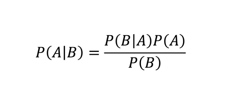
Image 1 shows Bayes’ theorem. P(A|B) is the posterior probability: the probability of A given B. P(B|A) is the likelihood, P(A) is the prior probability, and P(B) is the marginal likelihood, or evidence.
Logistic
The Logistic classifier’s core is the logistic function. WEKA’s classifier uses a multinomial logistic regression model with a ridge estimator.
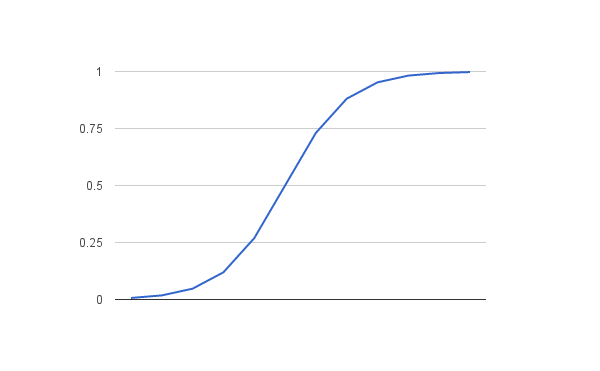
Image 2 represents the logistic function curve. Logistic regression combines input values linearly using learned weights or coefficients, then maps the result to a binary output. The logistic regression equation is y = e^(b0 + b1*x) / (1 + e^(b0 + b1*x)), where y is the predicted output, b0 is the bias or intercept term, and b1 is the coefficient for the input value.
IBk
The IBk classifier uses the k-nearest neighbours (KNN) algorithm.
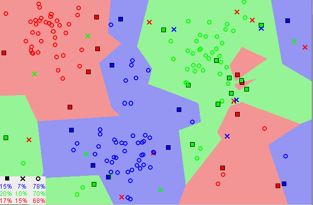
Image 3 shows a spread of data points. KNN captures similarity by calculating the distance between points, then voting for the most frequent label among the nearest neighbours. In this project, k was set to 1, which can create instability but improves efficiency.
Classification via regression
Classification via regression adapts regression methods for classification tasks. The class value is binarised as 1 or 0, and one regression model is built for each class. After training, the classifier predicts the likely outcome based on the learned models.
J48
J48, also known as C4.5, uses a top-down, recursive, divide-and-conquer method to identify strong splitting attributes. In this experiment, the algorithm attempts to separate “1” outcomes from “0” outcomes as cleanly as possible.
Consider a J48 tree trained on the outcomes of eight games: four wins and four losses. “1” and “0” denote wins and losses, respectively. A simplified split might look like this:
If total points > 100, outcome = 1, 1, 1, 0. (Subset 1)
If total points ≤ 100, outcome = 0, 0, 0, 1. (Subset 2)
A perfect split is unlikely because each game contains substantial uncertainty. J48 continues splitting the data until each subset is as clean as possible. In general, a smaller tree is preferable because it is easier to interpret and less likely to overfit. Once trained, the tree is evaluated using the test set, and precision, recall, and F-measure are calculated.
PART
The PART algorithm is similar to a J48 tree, but it builds partial decision trees and converts the best leaf into a rule at each iteration. Its main advantage is simplicity: it avoids the need for global optimisation, which can reduce training and testing time.